“Biological variation” is an easy explanation to reach for when repeated measurements don’t match up very well. It is vague enough to excuse inconsistency in nearly any biological experiment, and in many cases, it is difficult to disprove. But in cell counting, there is a well-characterized source of variation that has absolutely nothing to do with biology at all.
This variation or ‘noise’ is inherent to counting all sorts of independent events or objects. It affects the number of galaxies in a telescope image, the number of clicks in a Geiger counter in a given time period, and the number of bugs hitting a windshield. It is found in the number of photons hitting each pixel of a camera’s sensor, causing your photos to look all grainy and pixelated when you take selfies in a dark room. It also causes variation when cells in suspension are pipetted into a hemocytometer or are otherwise sampled for counting.
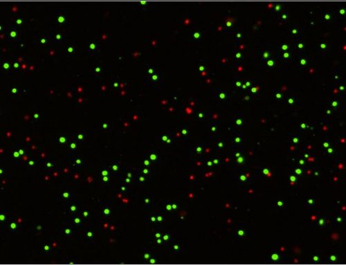
Let’s illustrate with a cell counting example. Suppose we have a hemocytometer, a wretched device that no one has ever enjoyed using. While there are various kinds of hemocytometers, they share the same basic form: a well-controlled gap between two pieces of glass with a grid pattern etched into one of the glass surfaces. We pipette some cell suspension into the gap, and cells fall like snow onto the grid. The cells are mixed well beforehand, and we exert no control whatsoever on where each cell will happen to land in the grid – they end up randomly scattered all over the glass.
Next, a sampling area is chosen and the cells within the area are counted. Knowing the precise area within the grid and the gap between the glass we can easily work out the cell concentration. (Automated cell counters use a similar principle, counting the number of cells that happen to fall within the grasp of the sensor and returning a concentration.) But the question is, “If we take more cells and do it again, will we get the same concentration?”. The answer, unless we get incredibly lucky, is “no”. We can have perfect mixing, perfect pipetting, a perfect hemocytometer, and perfect ability to count the cells without any mistakes – and still, we will have variation. This is the Poisson noise. It has nothing to do with the cells being cells, and nothing to do with our ability to count them properly. It is a fundamental limitation to our precision, like the speed of light is to a spaceship. Understanding this aspect of cell counting is key to improving our results.
The key feature of Poisson noise is that it follows the Poisson distribution, in which the statistical variance is equal to the mean number of objects counted (Figure 1). So, if we load the perfect hemocytometer many times from the same well-mixed suspension, and we happen to count an average of 100 cells per count, the variance in our counts will be 100 and the standard deviation will be its square root: 10 cells. Expressed as a relative uncertainty or coefficient of variation, we have a coefficient of variation (CV) of 10%.

Figure 1. Example normal distribution showing probability of results within certain standard deviation. The number of objects counted will impact the width of the distribution. The more objects are counted, the narrower the distribution indicating higher precision.
While the standard deviation becomes larger when more cells are counted, it grows more slowly than the number of objects itself, so the relative uncertainty (CV) becomes smaller with more counted objects.
To reduce the impact of Poisson noise, count as many cells as possible. The Poisson noise will decrease according to CV=√n/N=1/√n.
The Poisson noise represents the performance of a perfect cell counting process – the best that can be done using a random sampling technique, but it is actually possible to observe CVs that are smaller than the Poisson noise in real experiments. How? The answer is that when a small number of measurements are taken, we can get lucky. Like rolling a die and getting a 6 several times in a row, we may sometimes get cell counts that are more similar than probability would predict. Of course, we could just as easily be unlucky, obtaining a CV that is much larger than expected by pure chance. However, the more measurements we take, the (less fuzzy) the Poisson (speed limit) becomes. If an experiment is done with say 100 replicates, it would be highly unlikely to see a CV much lower than the Poisson limit.
So how should we think about real cell counting methods? After all, as highly as we may regard our pipetting skills, there may still be some variation introduced. Instruments, consumables, and counting analysis/algorithms may all contribute variation. In practice, these factors combine to create a ‘noise floor’ for the cell counting method, meaning that the CV will not drop below a certain level regardless of how many objects we count (Figure 2). The strategy, then, is to count as many objects as possible up to the point where the noise floor becomes the dominant source of variation.

Figure 2. An example CV prediction plot of cell counting experiments. If only 100 cells are counted, such as in a hemocytometer, a CV of 10% can be expected without other errors from sample preparation. As the number of cells counted increases, the CV can decrease to approximately 2% at 10,000 cells.
How do we count more objects? It depends on the specific case. Sometimes the original suspension that we want to measure is far too concentrated for direct cell counting (e.g., blood) and requires dilution. Other times, cells may come to us at exceptionally low concentrations. If either dilution or centrifugation of a sample is required, it is often best to target the high end of the range for which the cell counting instrument is designed. For manual counting, about 100 cells may be counted at a time to reduce the difficulty for the operator, but occasionally dilution protocols that are designed for manual counting are inadvertently left in place when an automated counting method is implemented. This means the samples are diluted more than necessary and the Poisson noise is higher than it could be. In short, don’t use your automated cell counter to count hundreds of cells if it can count thousands well (Figure 3).

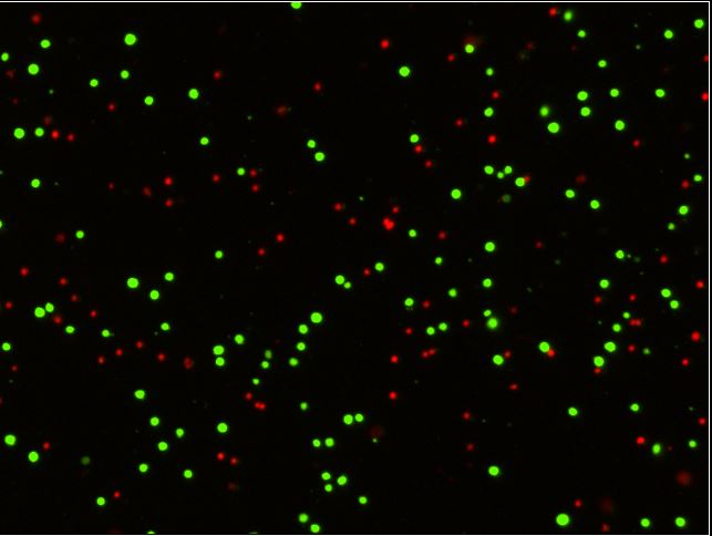
Figure 3. Example data of beads counted using the Cellaca MX high-throughput cell counter at various concentrations. It is obvious that higher concentrations showed smaller standard deviations in comparison to the lower concentration samples.
In some cases, you may be stuck with cells at a low concentration. One easy trick to improve precision is to average multiple independent measurements into a new measurement. In the case of a perfect cell counting method, the Poisson Noise of these new measurements will be the same as if a single measurement was made at a concentration high enough to count the same number of objects. For example, each measurement at 100x concentration will have the same uncertainty as the average of 10 measurements at 10x concentration. For real-life cell counting methods, there are additional sources of variation, so this relationship does not hold exactly, but it’s still a good rule of thumb. At any rate, it is easy to estimate the minimum uncertainty of your measurements based on the number of objects you are counting.
Understanding Poisson noise on a basic level helps us to set proper expectations for our cell counting. It is impossible* to truly get 10% CVs when your method only counts 50 objects per measurement! This knowledge also helps us improve our cell counting by optimizing our protocols to count as many cells as accurately as possible.
*For independent measurements of randomly sampled objects.
We would like to acknowledge Jordan Bell for providing his expertise and knowledge to complete this blog.
References
- Bell J, Huang Y, Qazi H, Kuksin D, Qiu J, Lin B, Chan LL-Y. Characterizing a novel high-throughput, high-speed, high-precision plate-based image cytometric cell counting method. Cell and Gene Therapy Insights 2021;7:427-447.
- Huang Y, Bell J, Kuksin D, Sarkar S, Pierce LT, Newton D, Qiu J, Chan LL-Y. Practical application of cell counting method performance evaluation and comparison derived from the ISO Cell Counting Standards Part 1 and 2. Cell and Gene Therapy Insights 2021;7:937-960.
- Pierce L, Sarkar S, Chan LL-Y, Lin B, Qiu J. Outcomes from a cell viability workshop: fit-for-purpose considerations for cell viability measurements for cellular therapeutic products. Cell and Gene Therapy Insights 2021;7:551-569.
- Siavash Ghavami, Olaf Wolkenhauer, Farshad Lahouti, Mukhtar Ullah,Michael Linnebacher. Accounting for randomness in measurement and sampling in studying cancer cell population dynamics. IET Systems Biology 2014;8(5):230-241


Leave A Comment